WP121.130 Exercise#2 Report

Abstract

The main objective of this exercise is to analyse the numerical convergence of the frequency computations for the different oscillation codes. To do so we compute the oscillations (p modes) from the same 001 and 002 models of exercise#1 but with different number of shells (2K, 4K, 6K, 8K, 16K) and mesh redistribution using ADIPLS routines. These routines also verify that HE and BV tests are passed.

1 The models

For this exercise we use the same modelS of exercise#1, computed with GARSTEC (provided by Jørgen). Details and physics at the Wiki site.

No	Mass	FeH	alpha	dov	Nshell	Phase
001	1.04	+0.00	2	0.00	P00-P16	MS
002	1.04	+0.00	2	0.00	P00-P16	MS

Table 1: List of models used in exercise#2. P00-P16 stands for the range of redistributed models with different number of mesh points. The range goes from the original (P00) up to 16k mesh pints (P16) through P02, P04, P06, and P08, which correspond with 2K, 4K, 6K, and 8K mesh points, respectively.

2 The oscillation codes

Here we list the all the participants and the main characteristics of their oscillation computation (code, numeric approach, etc.)

code	ver	EF	IS	Ri	IV	G	Prov
ADIPLS	0.3	P'	2,4	n	r	6.67232	AS
GraCo	R	P'/dP	2	y	r, r/P	6.67428	AM
GYRE	5.1	P'	2,4,6	n	r	6.67232	KD

Table 2: Main characteristics of the codes involved in exercise #1: ver stands for the code version, EF stands for EigenFunction variable (Eulerian P’, Lagrangian dP); IS stands for Integration Scheme; Ri stands for Richardson extrapolation; IV stands for integration variable (r or r/P); Rm stands for remeshing; G is the Universal gravitation constant (format D-8), and Prov stands for provider of the frequencies (name acronym).

Note

The official value for the gravitational constant was fixed by the consortium to be \(G = 6.6743\,10^{-8} (cgs)\). The fact of using different values for G by the codes is not relevant for the exercise, since there is no inter-comparison of codes.

3 Numerical convergence of the frequencies

Following the conclusions of exercise#1, the oscillation frequencies are computed with a fourth-order integration scheme or equivalent (e.g. O(2)+Rich for GraCo).

From that exercise we also found that we still need to explore the suitability of eulerian/lagrangian integration variable, so here frequencies are computed by (GYRE and GraCo) for both cases (ADIPLS has no lagrangian option). We compute all the mode from n \(n=1\) to the cut-off frequency, although we focus around the solar \(\nu_{\mathrm{max}}= 3090\,\mu{\mathrm{Hz}}\), i.e. around \(n=20-21\).

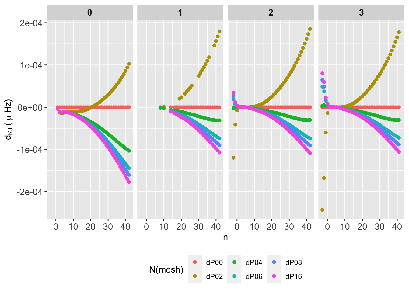
We study the numerical convergence of frequencies analyzing the evolution of each individual frequency with the number of mesh points. In practice, we compute the difference between each frequency for each \(\nu(n,\ell,K)\) with a reference frequency, e.g. \(\nu(n,\ell,P00=5K)\), that is

\[ D_{K,J} = \nu(n,\ell,K) - \nu(n,\ell,J), \tag{1}\]

for the absolute frequency difference, and

\[ d_{K,J} = \frac{\nu(n,\ell,K) - \nu(n,\ell,J)}{\nu(n,\ell,J)}. \tag{2}\]

for the relative frequency difference. The \(K\) index represents the different number of mesh points (P00, P02, etc.) and \(J\) is the reference number of mesh points (e.g. P00).

3.1 The Eulerian case

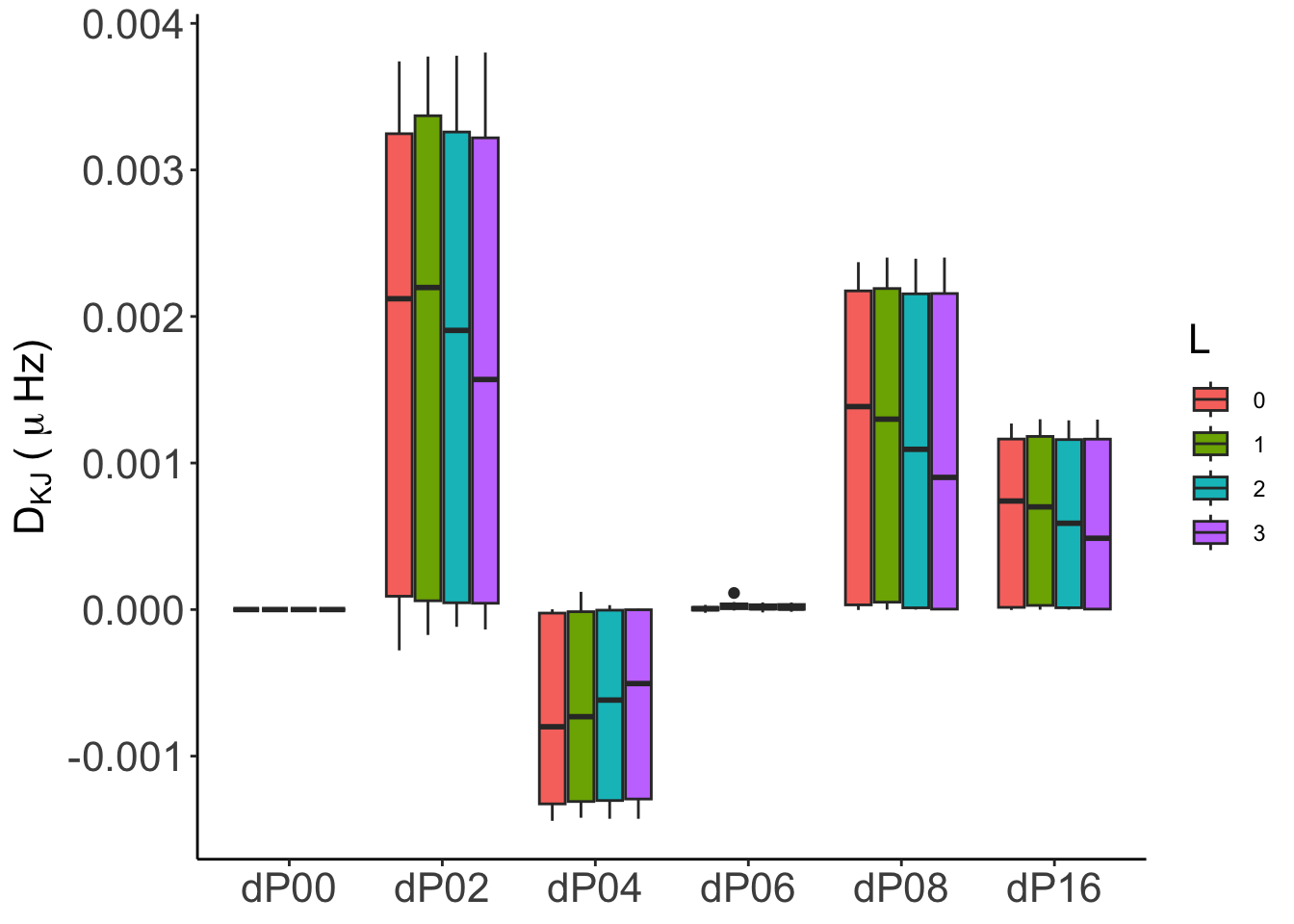
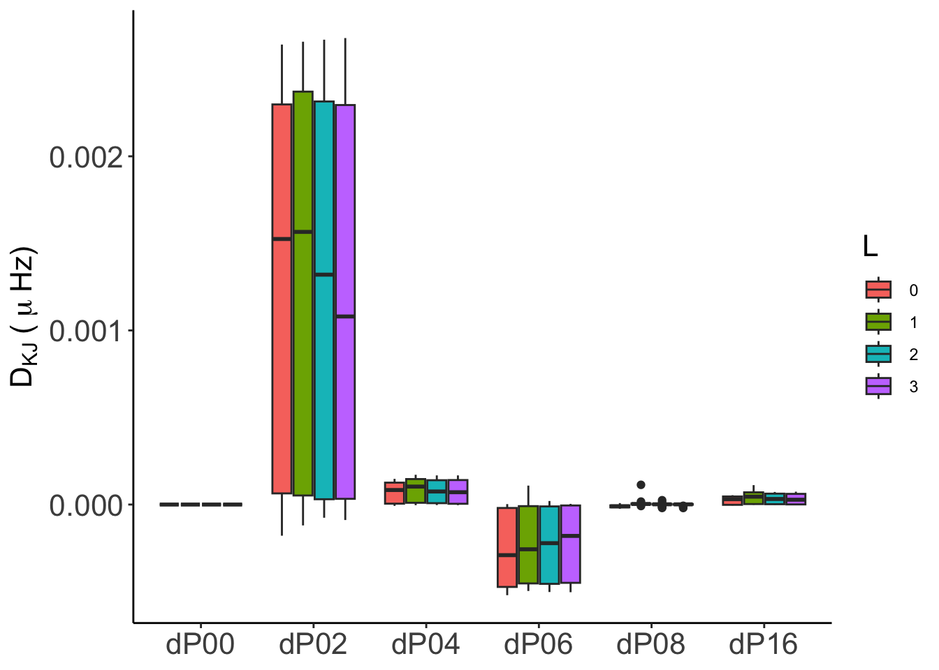
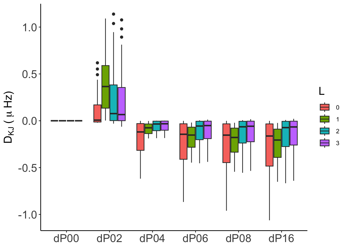
This is the most complete case, since the Eulerian variable option is covered by the three codes. The following tab-like figures show the absolute and relative frequency differences \((D_{K,J}, d_{K,J})\), as well as the statistics for \(D_{K,J}\) under the form of boxplots.

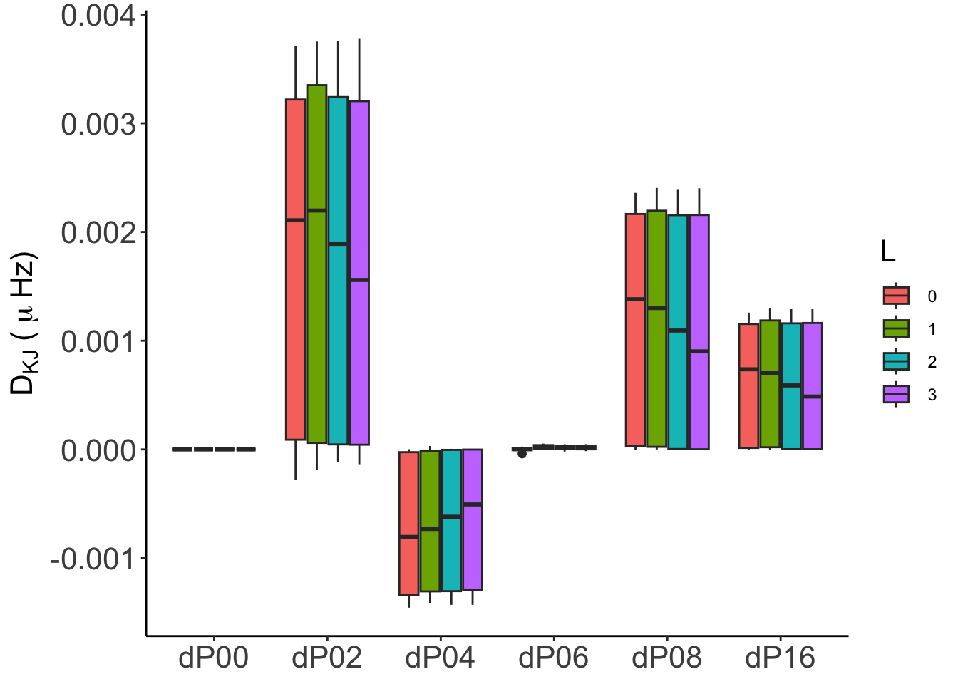
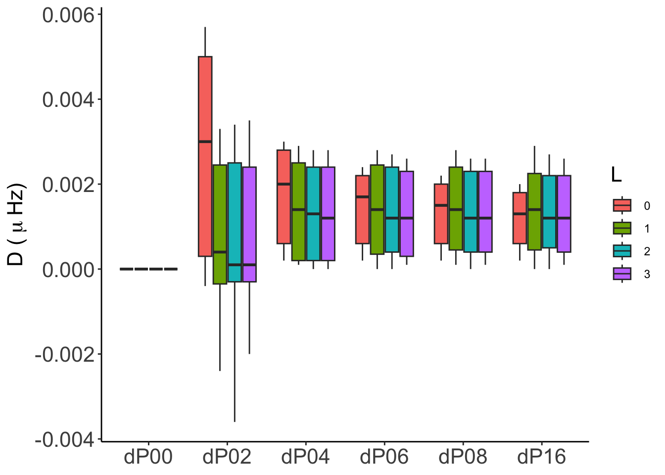
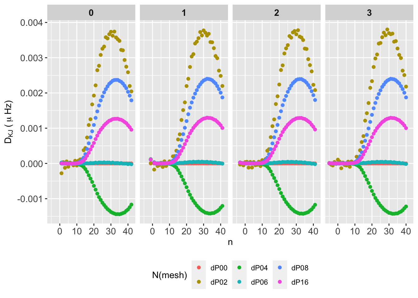
Figure 1: \(D_{KJ}\) (Eq. 1) computed for GYRE on model 2-001, with ref P00.

The behaviour is identical for all mode degrees. Differences are all postive except for P06. Differences grow for decreasing mesh points, as expected. All \(D_{KJ}\) remains below 0.004, and reach up \(0.002\,\mu\mathrm{Hz}\) around \(n=20\) as the worst case.

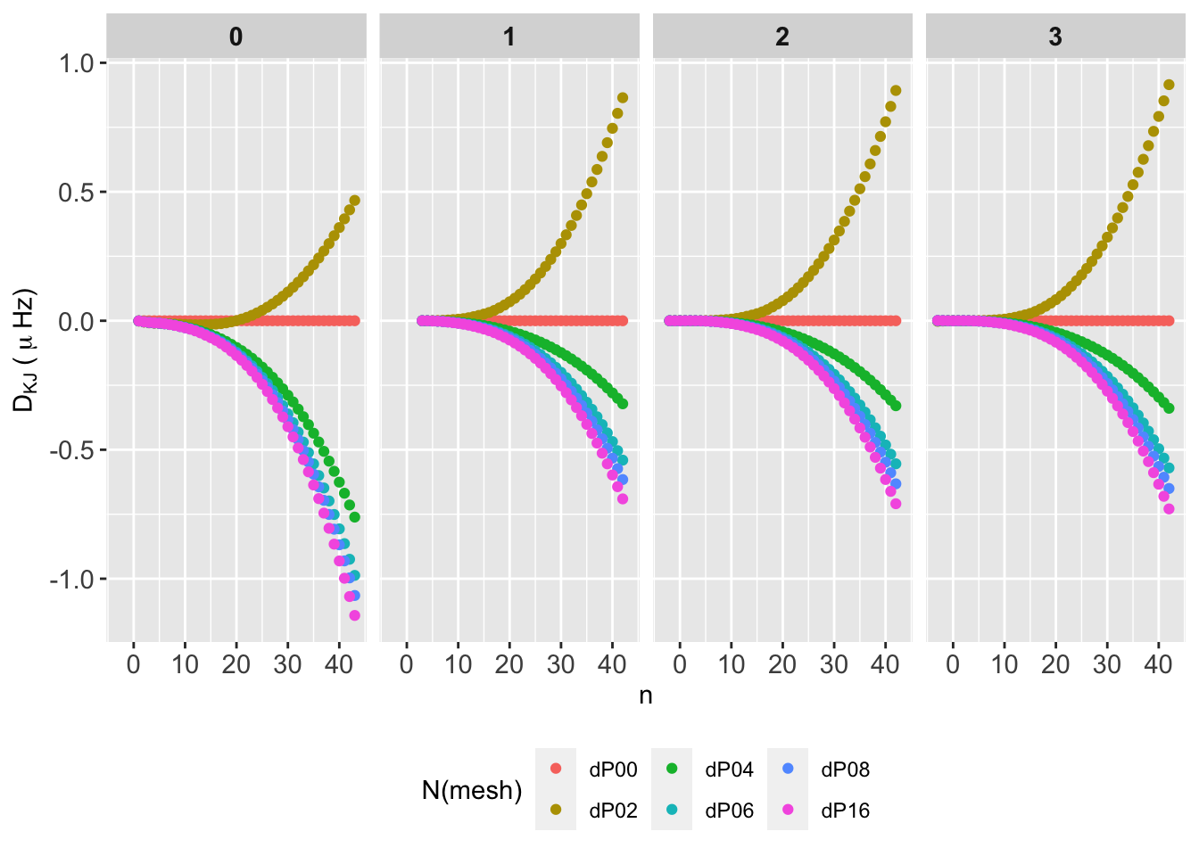
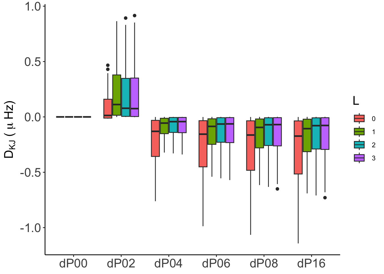
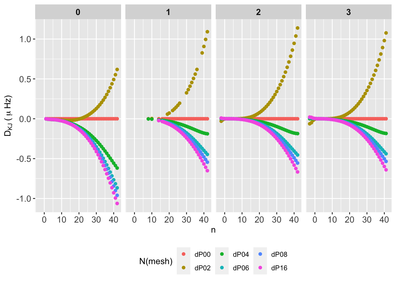
Figure 2: \(D_{KJ}\) (Eq. 1) computed for GraCo on model 2-001, with ref P00.

The behaviour is identical for all mode degrees. Differences are all negative except for P02, and grow for increasing mesh points, which may be due to the second order IS (tbc). \(D_{KJ}\) reach up to \(0.5\,\mu\mathrm{Hz}\) around \(\nu_{\mathrm{max}}\), up to \(0.5 \mu\mathrm{Hz}\) for \(n~[25,30]\), and up to \(1 \mu\mathrm{Hz}\) for \(n~40\).

Figure 3: \(D_{KJ}\) (Eq. 1) computed for ADIPLS on model 2-001, with ref P00.

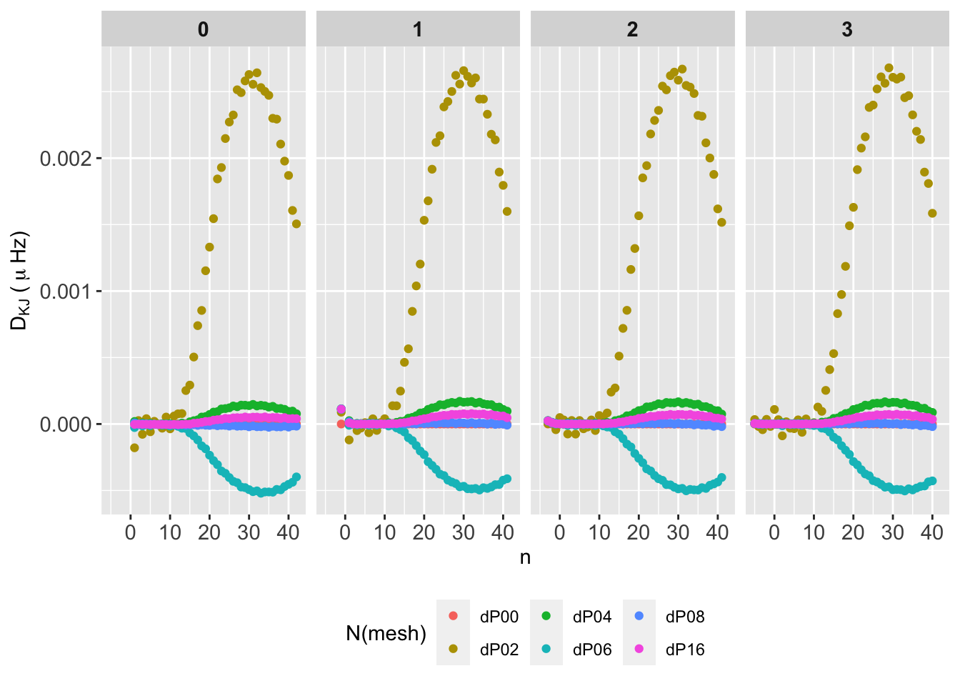
The behaviour is identical for \(\ell=1-3\). For \(\ell=0\) P02 frequencies seem to grow faster. Differences are all postive except for P02, which shows a sine-ish form, with \(D_{KJ}<0\) for \(n=1\) to \(n=10\) and \(D_{KJ}>0\) from \(n=10\) up to \(n=20\). From there, differeces drastically drecrasy up to negative values near \(n=40\). For the rest of cases, differences gentlty gro up to \(n=35\), where shows again a drastic drop. All \(D_{KJ}\) remains below 0.0055, and reach up \(0.0025\,\mu\mathrm{Hz}\) around \(n=20\) as the worst case.

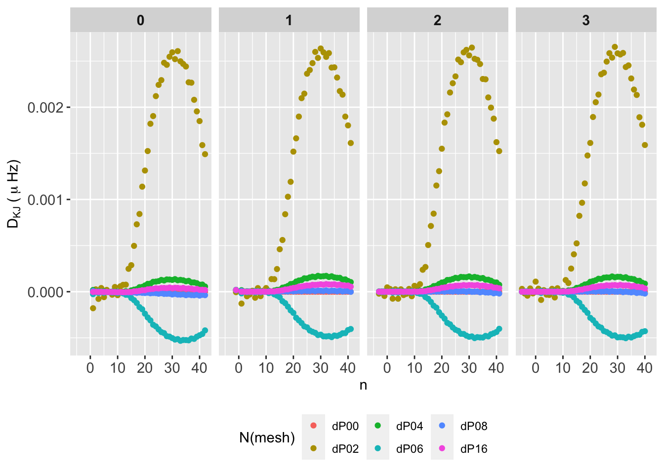
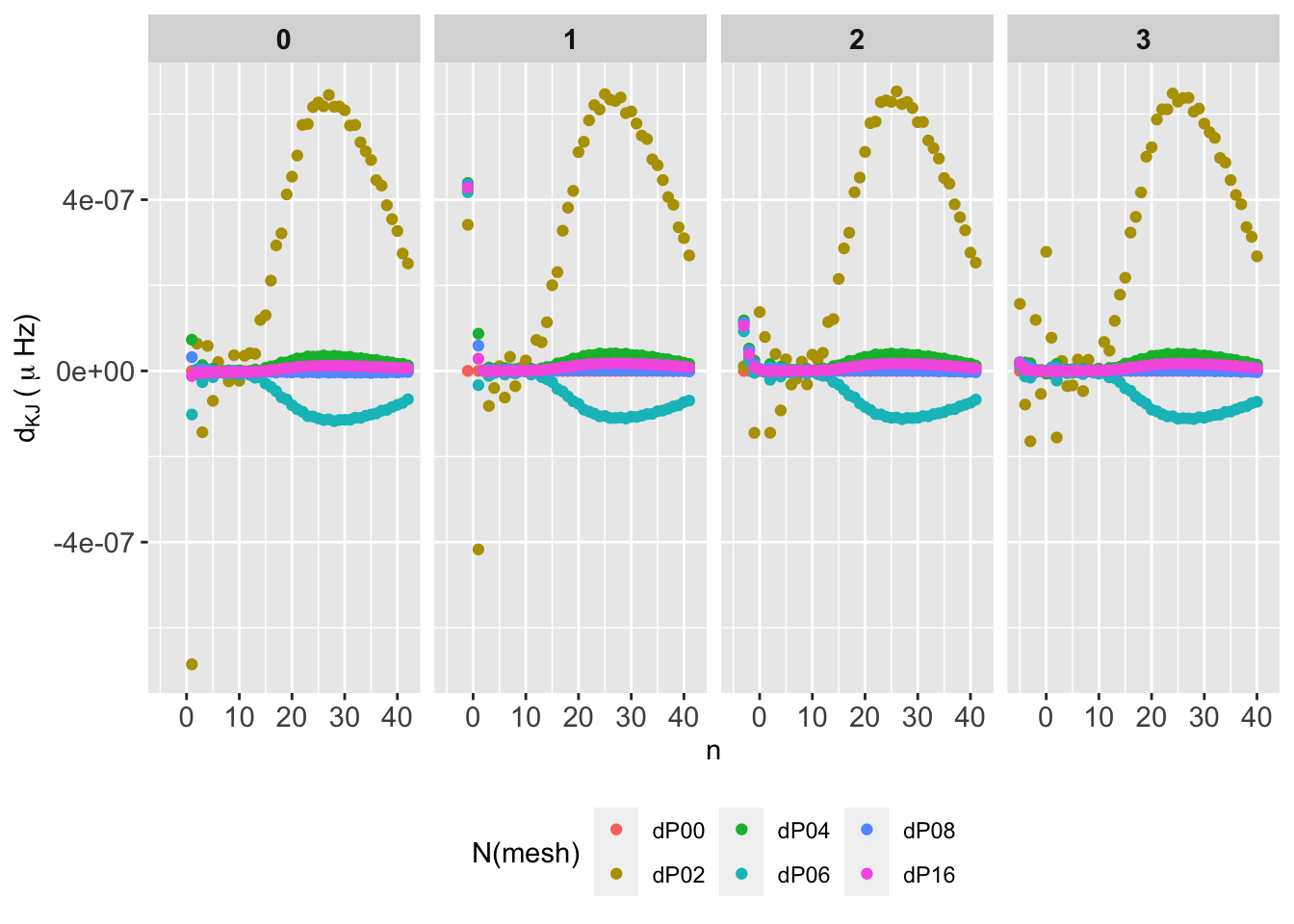
Figure 4: \(D_{KJ}\) (Eq. 1) computed for GYRE on model 2-002, with ref P00.

Similar results to those found for model 2-001 (see Fig. 1) with slight variations in the maximum differences.

Figure 5: \(D_{KJ}\) (Eq. 1) computed for GraCo on model 2-002, with ref P00.

Similar results to those found for model 2-001 (see Fig. 2) with slight variations in the maximum differences.

Figure 6: \(D_{KJ}\) (Eq. 1) computed for ADIPLS on model 2-002, with ref P00.

Similar results to those found for model 2-001 (see Fig. 3) with slight variations in the maximum differences.

Figure 7: \(d_{KJ}\) (Eq. 2) computed for GYRE on model 2-001, with ref P00.

Figure 8: \(d_{KJ}\) (Eq. 2) computed for GraCo on model 2-001, with ref P00.

Figure 9: \(d_{KJ}\) (Eq. 2) computed for ADIPLS on model 2-001, with ref P00.

Figure 10: \(d_{KJ}\) (Eq. 2) computed for GYRE on model 2-002, with ref P00.

Figure 11: \(d_{KJ}\) (Eq. 2) computed for GraCo on model 2-002, with ref P00.

Figure 12: \(d_{KJ}\) (Eq. 2) computed for ADIPLS on model 2-002, with ref P00.

Figure 13: Summary of statistics for \(D_{KJ}\) for the GYRE code.

Figure 14: Summary of statistics for \(D_{KJ}\) for the GraCo code.

Figure 15: Summary of statistics for \(D_{KJ}\) for the ADIPLS code.

Figure 16: Summary of statistics for \(D_{KJ}\) for the GYRE code.

Figure 17: Summary of statistics for \(D_{KJ}\) for the GraCo code.

Figure 18: Summary of statistics for \(D_{KJ}\) for the ADIPLS code.

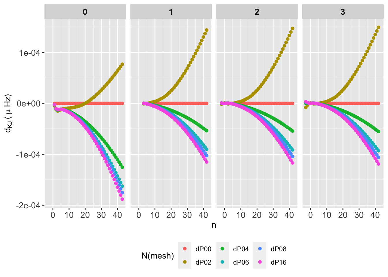
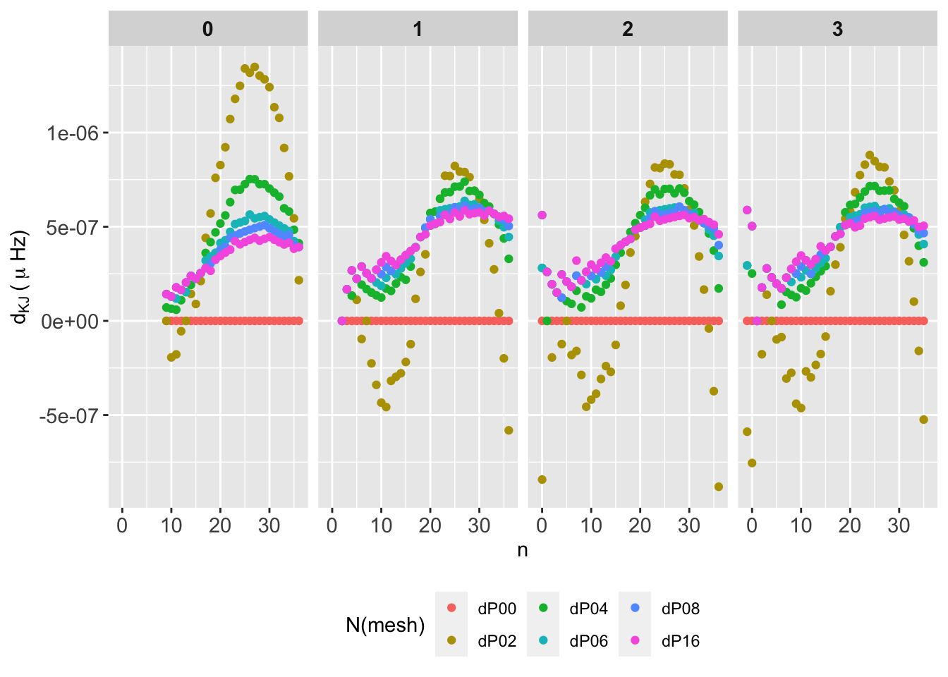
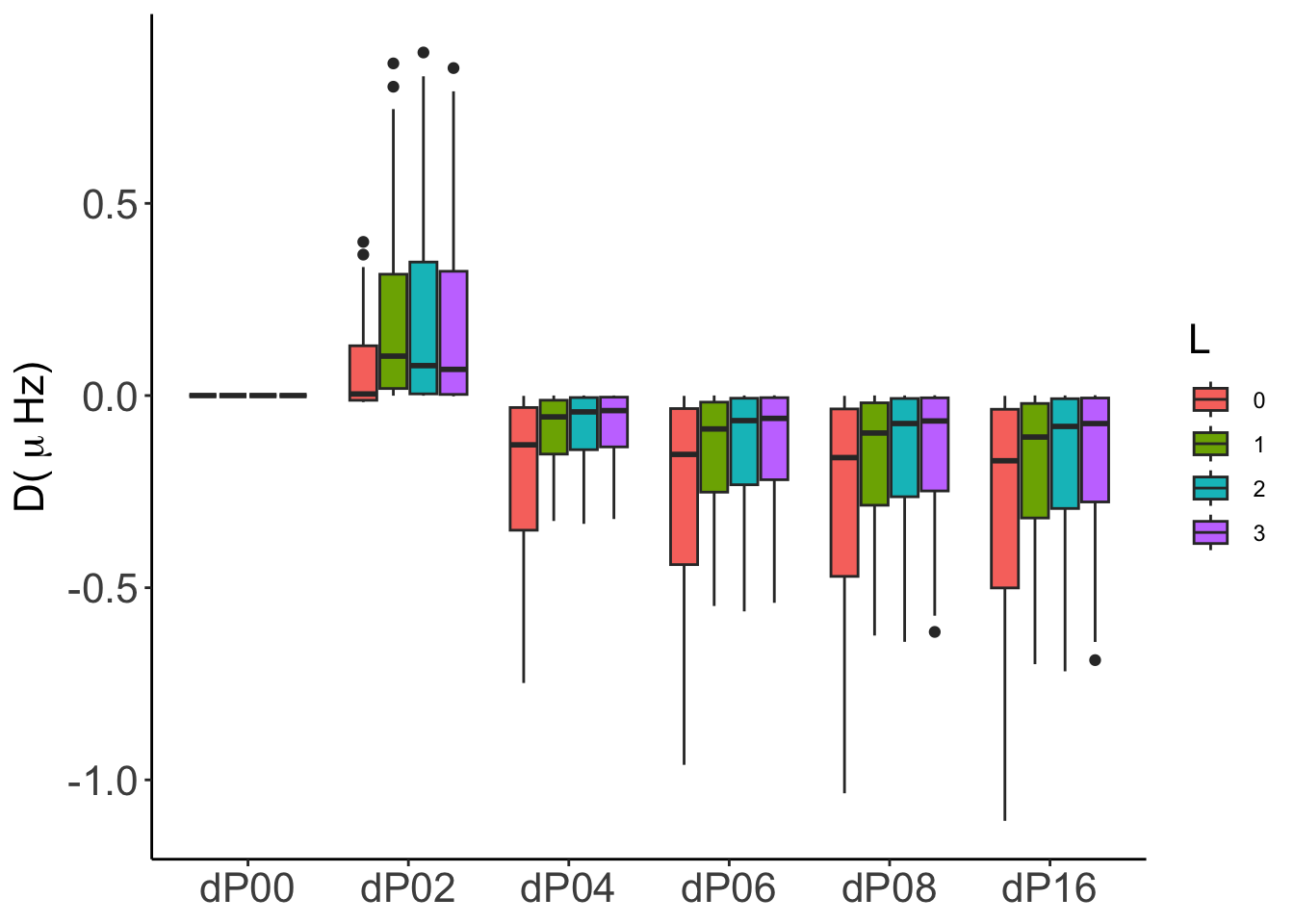
In general, both absolute (\(D_{KJ}\)) and relative (\(d_{KJ}\)) differences are numerically consistent, with differences below \(0.01\,\mu\mathrm{Hz}\) in all cases except for GraCo, whose frequency computations were made with IS(2). We will incorporate IS(4) results as soon as we have it, although, in any case we expect them to be similar to those shown by GYRE and ADIPLS.

For GYRE the statistics show that from P04, the numerical convergence is robust and reliable. In particular for P08 and P16, even considering all the frequency range, the distribution of probabilities are very close to the median with almost no outliers.

For ADIPLS there are almost no difference in the global statistical behaviour, being the P02 the worst case. From P04 on the median is around \(0.001-0.002\,\mu\mathrm{Hz}\) with no outliers.

For GraCo the stats a worse than for the other codes due to the same reason, frequencies are computed with IS(2). We’ll update this when IS(4) are provided for the analysis.

There are no significant differences between models 2-001 and 2-002.

3.2 The Lagrangian case

This case is only covered by GYRE and GraCo codes.

Figure 19: \(D_{KJ}\) (Eq. 1) computed for GYRE on model 2-001, with ref P00.

Figure 20: \(D_{KJ}\) (Eq. 1) computed for GraCo on model 2-001, with ref P00.

Figure 21: \(D_{KJ}\) (Eq. 1) computed for GYRE on model 2-002, with ref P00.

Similar results to those found for model 2-001 (see Fig. 19) with slight variations in the maximum differences.

Figure 22: \(D_{KJ}\) (Eq. 1) computed for GraCo on model 2-002, with ref P00.

Similar results to those found for model 2-001 (see Fig. 20) with slight variations in the maximum differences.

Figure 23: \(d_{KJ}\) (Eq. 2) computed for GYRE on model 2-001, with ref P00.

Figure 24: \(d_{KJ}\) (Eq. 2) computed for GraCo on model 2-001, with ref P00.

Figure 25: \(d_{KJ}\) (Eq. 2) computed for GYRE on model 2-002, with ref P00.

Figure 26: \(d_{KJ}\) (Eq. 2) computed for GraCo on model 2-002, with ref P00.

Figure 27: Summary of statistics for \(D_{KJ}\) for the GYRE code.

Figure 28: Summary of statistics for \(D_{KJ}\) for the GraCo code.

Figure 29: Summary of statistics for \(D_{KJ}\) for the GYRE code.

Figure 30: Summary of statistics for \(D_{KJ}\) for the GraCo code.

For GYRE the, as for the euleriancase, the statistics show that from P04, the numerical convergence is robust and reliable. In particular for P08 and P16, even considering all the frequency range, the distribution of probabilities are very close to the median with almost no outliers. The global statistical behaviour improve for model 2-002 from P04 on.

For GraCo the stats a worse than for the other codes due to the same reason, frequencies are computed with IS(2). We’ll update this when IS(4) are provided for the analysis.

4 Preliminary conclusions

The numerical convergence of the frequencies shown by GYRE and ADIPLS is robust and reliable. GraCo results are not representative (we will discuss them in detail when IS are delivered). The variations in the frequencies computed by these codes are around \(0.005\,\mu\mathrm{Hz}\) in the worst case, and around \(0.002\,\mu\mathrm{Hz}\) around \(n=20\).

P04 seems good for the frequency computations, although P06 is the optimum case (in terms of frequency differences). It worth study the impact of choosing P06 instead of P4 on the computation time.

As expected, model 2-002 gives slightly better global behaviour in the statistics.

The choice of eulerian/lagrangian variable has no significant impact on the results.